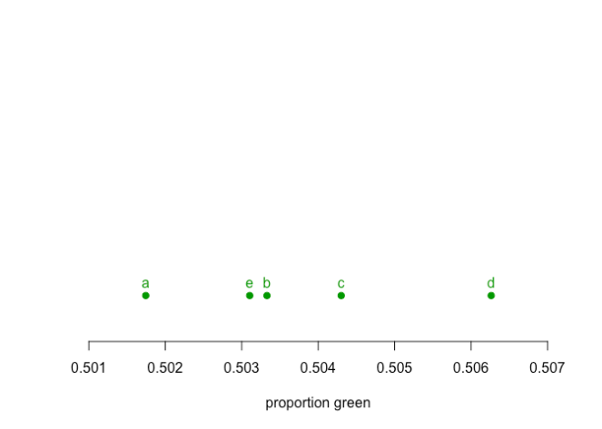
This is a short example of how aggregation of categorical variables creates false variation, which in turn creates misleading results in statistical tests for comparing variation (like Chi Squared, Fisher’s, or comparisons of proportions)
Let’s say we have a hypothetical set of values
| area | green | blue |
|---|---|---|
| a | 92194 | 91553 |
| b | 88504 | 87333 |
| c | 83836 | 82406 |
| d | 86249 | 84115 |
| e | 83954 | 82918 |
And we are interested in a question of is the group d unusually different to the other groups.
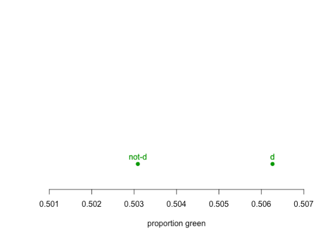
But if we aggregate the data to form a problem defined by the difference between d and not-d
| area | green | blue |
|---|---|---|
| d | 86249 | 84115 |
| notd | 348488 | 344210 |
suddenly d is looking very different from things that are not d
A formal Chi-Squared test of the differences between d and not-d gives p-value of 0.019, with a similar result from a Fisher’s Exact Test (0.0189), so we conclude that the difference between d and not-d is significant and thus reject the Null Hypothesis there is no difference.
On the other hand, if we carry out a Chi-Squared test on the original 5 groups, the p-value is 0.0968, which would be a failure to reject the Null Hypothesis at a 95% level of significance, thus we keep the Null Hypothesis there is no difference between the groups. If we carry out a set of post-hoc tests among the individual pairs with a Bonferroni multiple testing correction (which we should do even if the initial result was significant) we find there is a significant difference between group a and d, but the differences between d and b,c, or e are not significant. Logically, this must lead to a rejection that d is different to the set of (A,B,C,E).
This is a clear contradiction in results, using the same statistical test but on the aggregated and the unaggregated data. The reason for this is that the expected distribution of the aggregated data (the distribution of the aggregate) is not the same as the combined distributions of the individual groups (the aggregate of the distributions). Information about the differences between the individual groups is lost when the data is aggregated, so the distribution of the aggregate does not reflect the actual distribution.
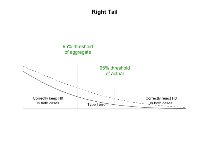
When the actual distribution of the data is wider (more varied) than the constructed distribution for the aggregate Type I errors occur as the Null Hypothesis is rejected more easily than it should be. When the actual distribution of the data is narrower (less varied) than the constructed distribution of the aggregate Type II errors occur as the Null Hypothesis is rejected less often than it should be. Either error is possible, for example depending on what type of confounders might be acting on the data that are not accounted for in the comparison.
In this particular case the actual data is more varied than the distribution of the aggregate, which has lead to a Type I error as the particular tests applied on the aggregate have fallen into the zone in which the error occurs.
The Probability distributions
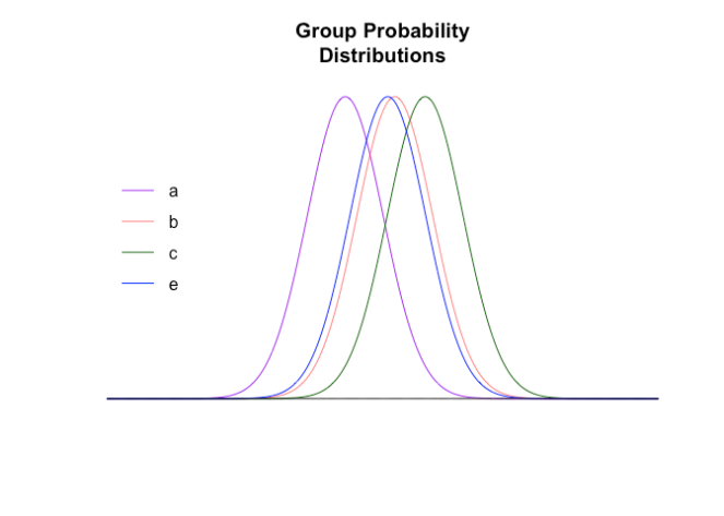
Fundamentally comparison tests are comparing distributions, and the distribution of the aggregated data is different to the aggregated distributions of the data. The expected distributions of the four non-d groups (graphically rendered using a proportion and a normal approximation to a binomial) are
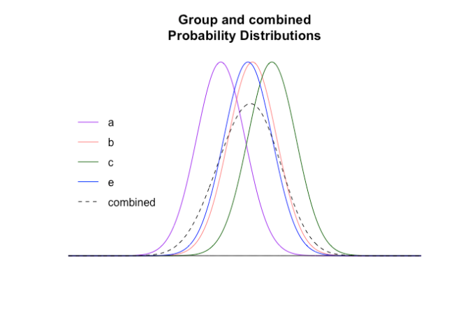
From this we can calculate the combined (actual) probability distribution of the groups
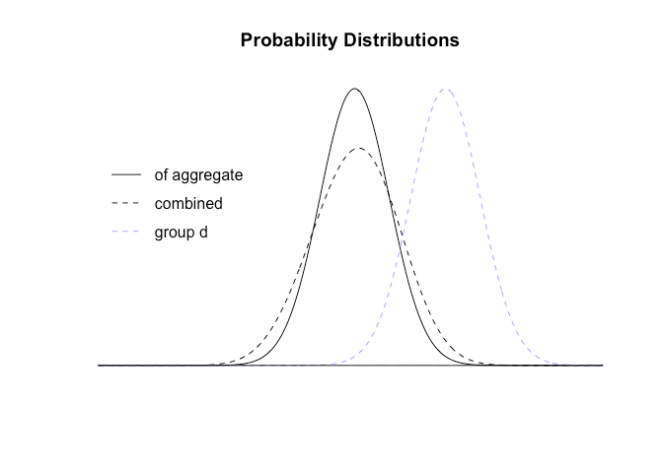
We can compare this distribution to the distribution of the aggregate (and show the distribution of group d as context)
These are very different distributions, so will give very different answers. If we zoom in on the right hand end representing the 95ht (two tailed) percentiles where results will be declared significant:
Chi squared
The above was showing the probability distributions using the normal approximation to the binomial simply because it was easy to graph. The same kind of aggregation error occurs with Chi Squared though I cannot make distribution graphs as easily, and it can be observed by starting with a distribution where entry d is at the marginal probabilities for the Null Hypothesis
| area | green | blue |
|---|---|---|
| a | 92194 | 91553 |
| b | 88504 | 87333 |
| c | 83836 | 82406 |
| d | 85708 | 84656 |
| e | 83954 | 82918 |
then shifting one entry for d at a time from the blue to green category and testing the p-values of the aggregated vs unaggregated values.
When green is 85819 (or lower) and blue is 84545 (or higher) the p value reported by the aggregate is higher than the unaggregated line and Type II errors occur. When green is 85820 (or higher) and blue is 84544 (or lower) the p value reported by the aggregate is lower than the unaggregated line and Type I errors occur.
The p value reduces below 0.05 for the aggregated data when green is 86161 (or higher) and blue is 84203 (or lower). This is the specific zone where the Type I error leads to a different conclusion when using a 95% level of significance. This wrong conclusion continues until the unaggregated p value results cross 0.05 when green is 86324 (or higher) and blue is 84040 (or lower). The actual data of green 86249, blue 84115 is in the middle of the Type I error range zone.
Independence
Most authorities warn against aggregating data because of the risk of violating independence assumptions, which are fairly fundamental to statistical tests. One way of thinking about it in this framework is that by combining cells in chi squared we are combining entries that have different unknown confounders acting on them causing different distributions, which is to say the data is not independent.
R code
finally, a bunch of R code to show my working
textdata <- '
"area", "green", "blue"
"a", 92194, 91553
"b", 88504, 87333
"c", 83836, 82406
"d", 86249, 84115
"e", 83954, 82918
'

fdata <- read.csv(text=textdata)

fdata$proportion_green = fdata$green / (fdata$green + fdata$blue)
stripchart(fdata$proportion_green, method = "stack", col="#009900", pch=19, offset=1,
           frame.plot=FALSE, xlim=c(.501,.507), ylim=c(0.5,4), xlab="proportion green")
text(x=fdata$proportion_green, y=c(1,1,1,1,1), labels=c("a","b","c","d","e"), pos=3, col="#009900")

wrong <- data.frame(area = c("d", "notd"),
                    green=c(fdata$green[4],sum(fdata$green[c(1:3,5)])),
                    blue=c(fdata$blue[4],sum(fdata$blue[c(1:3,5)])))

wrong$proportion_green = wrong$green / (wrong$green + wrong$blue)
stripchart(wrong$proportion_green, method = "stack", col="#009900", pch=19, offset=1,
           frame.plot=FALSE, xlim=c(.501,.507), ylim=c(0.5,4), xlab="proportion green")
text(x=wrong$proportion_green, y=c(1,1,1,1,1), labels=c("d", "not-d"), pos=3, col="#009900")

chisq.test(wrong[,2:3])
fisher.test(wrong[,2:3])
chisq.test(fdata[,2:3])

#divide significance threshold by 4 for the multiple testing correction
chisq.test(fdata[c(1,4),2:3])
chisq.test(fdata[c(2,4),2:3])
chisq.test(fdata[c(3,4),2:3])
chisq.test(fdata[c(5,4),2:3])
fisher.test(fdata[c(1,4),2:3])
fisher.test(fdata[c(2,4),2:3])
fisher.test(fdata[c(3,4),2:3])
fisher.test(fdata[c(5,4),2:3])

fdata$sd_green <- (170000  * fdata$proportion_green *(1 - fdata$proportion_green)) ^ 0.5
fdata$m_green <- 170000 * fdata$proportion_green

x <- seq(84000,87000,length=1000)

hxa <- dnorm(x,fdata$m_green[1],fdata$sd_green[1])
plot(x, hxa, type="n", xlab="", ylab="",
  main="Group Probability\nDistributions", axes=FALSE, xlim=c(84000,87000))
lines(x, hxa, col="purple")

hxb <- dnorm(x,fdata$m_green[2],fdata$sd_green[2])
lines(x, hxb, col="#FF000099")

hxc <- dnorm(x,fdata$m_green[3],fdata$sd_green[3])
lines(x, hxc, col="darkgreen")

hxe <- dnorm(x,fdata$m_green[5],fdata$sd_green[5])
lines(x, hxe, col="blue")

lines(x, rep(0, times=1000))

legend(x=84000, y=0.0015, legend=c("a", "b", "c", "e"), lwd=1, col= c("purple", "#FF000099", "darkgreen", "blue"), bty="n", y.intersp=1.5, lty=c(1,1,1,1))

plot(x, hxa, type="n", xlab="", ylab="",
  main="Group and combined\nProbability Distributions", xlim=c(84000,87000), axes=FALSE)
lines(x, hxa, col="purple")

lines(x, hxb, col="#FF000099")

lines(x, hxc, col="darkgreen")

lines(x, hxe, col="blue")

hx1235 <- (hxa+hxb+hxc+hxe)/4
lines(x, hx1235, lty=2)

lines(x, rep(0, times=1000))

legend(x=84000, y=0.0015, legend=c("a", "b", "c", "e","combined"), lwd=1, col= c("purple", "#FF000099", "darkgreen", "blue", "black"), bty="n", y.intersp=1.5, lty=c(1,1,1,1,2))

wrong$sd_green <- (170000  * wrong$proportion_green *(1 - wrong$proportion_green)) ^ 0.5
wrong$m_green <- 170000 * wrong$proportion_green

hxagg <- dnorm(x,wrong$m_green[2],wrong$sd_green[2])
plot(x, hxagg, type="n", xlab="", ylab="",
  main="Probability Distributions", axes=FALSE, xlim=c(84000,87000))
lines(x, hxagg)
lines(x, hx1235, lty=2)

hxd <- dnorm(x,fdata$m_green[4],fdata$sd_green[4])
lines(x, hxd, col="#AAAAFF", lty=2)

legend(x=84000, y=0.0015, legend=c("of aggregate", "combined", "group d"), lty=c(1,2,2), bty="n", y.intersp=1.5, col=c("black", "black", "#AAAAFF"))

lines(x, rep(0, times=1000))

plot(x, hxagg, type="n", xlab="", ylab="",
  main="Right Tail", axes=FALSE, xlim=c(85800,86200))
lines(x, hxagg)
lines(x, hx1235, lty=2)
lines(x, rep(0, times=1000))


a95 <-qnorm(p=0.975, mean = wrong$m_green[2], sd = wrong$sd_green[2], lower.tail = TRUE, log.p = FALSE)
lines(c(a95,a95), c(0,0.001), col="#008800")
cumprob <- cumsum(hx1235) * 3
shortlist <- (cumprob[cumprob >= 0.975])
lines(c(x[cumprob == shortlist[1]],x[cumprob == shortlist[1]]), c(0,0.0005), col="#008800", lty=2)
text(x=a95, y=0.0014, labels="95% threshold\nof aggregate", col="#008800")
text(x=86027, y=0.0009, labels="95% threshold\nof actual", col="#008800")
text(x=85850, y=0.0002, labels="Correctly keep H0\nin both cases", cex=0.8)
text(x=85980, y=0.0001, labels="Type I error", cex=0.8)
text(x=86150, y=0.0002, labels="Correctly reject H0\nin both cases", cex=0.8)

textdata <- '
"area", "green", "blue"
"a", 92194, 91553
"b", 88504, 87333
"c", 83836, 82406
"d", 85708, 84656
"e", 83954, 82918
'
cdata <- read.csv(text=textdata)

gd <- 85708
bd <- 84656
i = 0:999
cresult <- data.frame(gd = i, bd = i, pagg = i, punagg = i)
for (j in 1:1000){
  cdata[4,2] <- gd + i[j]
  cdata[4,3] <- bd - i[j]
  cresult$gd[j] <- gd + i[j]
  cresult$bd[j] <- bd - i[j]
  wrong <- data.frame(area = c("d", "notd"),
                    green=c(cdata$green[4],sum(cdata$green[c(1:3,5)])),
                    blue=c(cdata$blue[4],sum(cdata$blue[c(1:3,5)])))
  cresult$pagg[j] <- chisq.test(wrong[,2:3])$p.value
  cresult$punagg[j] <- chisq.test(cdata[,2:3])$p.value
}

plot(cresult$gd,cresult$pagg, type="l", xlab="number green", ylab="reported pvalue", frame.plot=FALSE)
lines(cresult$gd,cresult$punagg, lty=2)
legend(x=86500, y=0.8, legend=c("of aggregate", "unaggregated"), lty=c(1,2), bty="n", y.intersp=1.5, col=c("black", "black"))
abline(v=86161, col="red")
abline(v=86324, col="red")
text(x=86230, y=0.8, labels="Wrong\nconclusion\ndue to\nType I error", col="red", cex=0.8)
points(86249,0.06, pch=19, col="#AAAAFF" )
text(x=86249, y=0.06, labels="Actual\nData", col="#AAAAFF", cex=0.8, pos=3)